2023. 2. 9. 11:58ㆍ기술 공부/Seaborn
+ Seaborn의 User guide and tutorial를 필사한 내용입니다.
+ 실행 환경은 Anaconda, IPython, Jupyter NoteBook 입니다.
오늘 다룰 주제는,
세 번째 글인 Multivariate views on complex datasets 이다.
바로 시작해보자.
오늘 글의 제목은 '복잡한 데이터 세트에 대한 다변량 보기'이다.
일부 seaborn 함수는 여러 종류의 플롯을 결합하여 데이터 세트에 대한 정보 요약을 신속하게 제공합니다. 하나, jointplot()는 단일 관계에 중점을 둡니다. 각 변수의 데이터 분포와 함께 두 변수 간의 데이터 분포를 플로팅합니다.
Some seaborn functions combine multiple kinds of plots to quickly give informative summaries of a dataset. One, jointplot(), focuses on a single relationship. It plots the joint distribution between two variables along with each variable’s marginal distribution:
오늘 글에서는 두 데이터에 대한 플롯을 그리는 내용인게 확실해 보인다.
하나라고 숫자를 세는 것을 보니 일단 한가지 방법은 아닌 것 같다.
jointplot()은 단일 관계에 중점을 둔다고 한다. 아마 1:1 관계를 말하는 것 같다.
jointplot()은 각 변수의 데이터 분포와 함께 두 변수 간의 데이터 분포를 띄운다고 한다.
음.. 두 데이터를 함께 볼 수 있게 잘 그려준다는 의미인 것 같다.
바로 한번 그려보자.
새로운 데이터 셋인 'penguins'를 불러왔다.
penguins = sns.load_dataset('penguins')penguins
sns.jointplot(
    data=penguins,
    x='flipper_length_mm',
    y='bill_length_mm',
    hue='species'
);
'fillper_length_mm'와 'bill_length_mm' 에 대한 species(종 분류)의 분포를 나타내는 플롯이 그려졌다.
또한 'fillper_length_mm', 'bill_length_mm' 각각의 데이터 분포도 위와 오른쪽에 그려졌다.
다른 하나인 pairplot()은 더 넓은 관점을 취합니다. 모든 데이터 쌍의 관계와 각 변수에 대한 분포를 각각 보여줍니다.
The other, pairplot(), takes a broader view: it shows joint and marginal distributions for all pairwise relationships and for each variable, respectively:
이번에 알아볼 pairplot()은 더 넓은 관점에서 데이터를 플로팅한다고 한다.
모든 데이터 쌍의 관계와 각 변수에 대한 분포를 보여준다는 말을 보아서,
1:1 관계 뿐만 아니라 n:n의 데이터 분포를 볼 수 있을 것으로 보인다.
sns.pairplot(
    data=penguins,
    hue='species'
);
뭔가 휘황찬란하게 그려졌다. 이런 걸 그린다면 뭔가 있어보일 것 같다. ㅋㅋ ㅋ
자세히 들여다보면, jointplot()을 사용했을 때의 플롯이 모두 모여있는 것으로 보인다.
이번엔 소제목이 붙어있다.
수치 작성을 위한 하위 수준 도구
Lower-level tools for building figures
저번에 알아본 글 중에서 Seaborn이 High-Level API라는 것을 배웠다.
이번에는 그 High-Level API를 구성하고 있는 Low-Level의 툴(클래스나 함수 정도)를 보여준다는 것 같다.
이러한 도구는 축 수준 플로팅 함수를 그림의 레이아웃을 관리하는 개체와 결합하여 데이터 집합의 구조를 축 그리드에 연결하여 작동합니다 . 두 요소 모두 공용 API의 일부이며 코드 몇 줄만 더 추가하면 복잡한 그림을 만드는 데 직접 사용할 수 있습니다.
These tools work by combining axes-level plotting functions with objects that manage the layout of the figure,
linking the structure of a dataset to a grid of axes. Both elements are part of the public API, and you can use them directly to create complex figures with only a few more lines of code:
흠. 이게 대체 무슨 소리일까. 하나씩 짤라서 이해해보자.
몇 가지를 짤라왔다.
- 그림: 플롯을 의미한다.
- 축 수준: 플롯은 x, y를 가지고 있다. 플롯을 구성하는 단위인 x, y 축을 의미한다.
- 플로팅 함수: 플롯을 화면에 띄우는 함수를 의미한다. relplot(), jointplot() 도 여기에 해당한다.
- 축 수준 플로팅 함수: x, y 축을 플로팅하는 함수를 의미하는 듯 하다.
여기서 PairGrid는 하나의 큰 플롯 안의 x, y 축에 여러 개의 작은 플롯을 소유한다.
축 수준 플로팅 함수는 PairGrid(하나의 큰 플롯) 내부의 x, y 축에 들어갈 작은 플롯을 그리는 함수가 되겠다.
또한 플로팅 함수가 relplot(), jointplot() 등등 을 포함하고 있으니,
relplot(), jointplot() 등등으로 PairGrid를 채우는 방법도 존재하지 않을까 한다.
- 그림의 레이아웃을 관리하는 개체: FacetGrid, PairGrid, JointGrid 등을 의미한다.
짤라진 것들을 조합해보면,
하나의 큰 그림(이하, 플롯)을 그리는 PairGrid에
작은 그림들을 그리는 relplot(), jointplot() 등을 이용해서,
내가 원하는 그림들을 그릴 수 있다는 이야기인 것 같다.
+ 내가 원하는 그림들을 여러개도 그릴 수 있다는 이야기인 것 같다.
먼저 코드가 여러 줄이므로,
각 코드가 어떤 역할을 하는 지 알기 위해 inline 백엔드 사용을 해지했다.
plt.ioff()
PairGrid를 생성하였다.
pair_grid = sns.PairGrid(
    penguins,
    hue='species',
    corner=True
)
plt.show()
여기서 plt.show()를 하게되면 pair_grid를 플로팅한 외부 창이 생성되고,
IPython은 이 플로팅된 외부 창의 백엔드(matplotlib)의 커널을 읽어와서 Cell에 출력한다.
그리고, 아래 코드에서 plt.show()를 실행하게되면,
이미 pair_grid가 플로팅되어 있는 외부 창이 닫히게 되므로, Cell에는 아무것도 출력되지 않는다.
(pair_grid에 그려야 하는데, pair_grid가 사라지게 되므로 아무 작동도 하지 않는다.)
pair_grid.map_lower(
    sns.kdeplot,
    hue=None,
    levels=5,
    color='.2'
)
plt.show()
따라서, 이렇게 Cell 2개를 실행해야 결과를 볼 수 있다.
pair_grid = sns.PairGrid(
    penguins,
    hue='species',
    corner=True
)
# plt.show()
pair_grid.map_lower(
sns.kdeplot,
hue=None,
levels=5,
color='.2'
)
plt.show()
비어있던 PairGrid에 지형도 같은게 그려졌다.
kdeplot이므로, 데이터 분포에 대한 커널 밀도를 표현한 것 같다.
또한 hue를 없애면, 커널 밀도가 (3개종에 대한 데이터이므로) 3개로 나누어진다.
즉, None 값을 전달하여 3개종에 대한 커널 밀도를 하나로 합친 것으로 보여진다.
levels는 최대 5개의 동그라미(?)까지 표현하라는 의미인 것 같다.
pair_grid = sns.PairGrid(
    penguins,
    hue='species',
    corner=True
)
# plt.show()
pair_grid.map_lower(
sns.kdeplot,
hue=None,
levels=5,
color='.2'
)
# plt.show()pair_grid.map_lower(
sns.scatterplot,
marker='+'
)
plt.show()
이번에는 점들이 '+' 모양으로 추가되었다.
pair_grid = sns.PairGrid(
    penguins,
    hue='species',
    corner=True
)
# plt.show()
pair_grid.map_lower(
sns.kdeplot,
hue=None,
levels=5,
color='.2'
)
# plt.show()pair_grid.map_lower(
sns.scatterplot,
marker='+'
)
# plt.show()pair_grid.map_diag(
sns.histplot,
element='step',
linewidth=0,
kde=True
)
plt.show()
이번엔 각 코너에 히스토그램과 커널 밀도가 생겨났다.
pair_grid = sns.PairGrid(
    penguins,
    hue='species',
    corner=True
)
# plt.show()
pair_grid.map_lower(
sns.kdeplot,
hue=None,
levels=5,
color='.2'
)
# plt.show()pair_grid.map_lower(
sns.scatterplot,
marker='+'
)
# plt.show()pair_grid.map_diag(
sns.histplot,
element='step',
linewidth=0,
kde=True
)
# plt.show()pair_grid.add_legend(
frameon=True
)
plt.show()
범례가 추가되었다.
pair_grid = sns.PairGrid(
    penguins,
    hue='species',
    corner=True
)
# plt.show()
pair_grid.map_lower(
sns.kdeplot,
hue=None,
levels=5,
color='.2'
)
# plt.show()pair_grid.map_lower(
sns.scatterplot,
marker='+'
)
# plt.show()pair_grid.map_diag(
sns.histplot,
element='step',
linewidth=0,
kde=True
)
# plt.show()pair_grid.add_legend(
frameon=True
)
# plt.show()pair_grid.legend.set_bbox_to_anchor((.61, .6))
plt.show()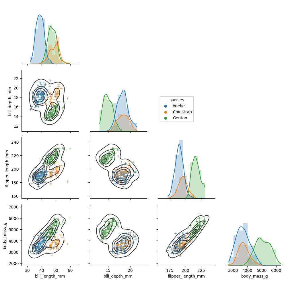
범례가 안쪽 좌표로 이동해왔다.
즉, 이런 방식으로 Grid를 이용하여,
하나씩 내가 원하는 것들을 그려나갈 수 있다는 의미인 것 같다.
출처 :
User guide and tutorial — seaborn 0.12.2 documentation
https://seaborn.pydata.org/tutorial/introduction.html#multivariate-views-on-complex-datasets
An introduction to seaborn — seaborn 0.12.2 documentation
An introduction to seaborn Seaborn is a library for making statistical graphics in Python. It builds on top of matplotlib and integrates closely with pandas data structures. Seaborn helps you explore and understand your data. Its plotting functions operate
seaborn.pydata.org
GitHub :
MoonsRainbow/seaborn-tutorial
https://github.com/MoonsRainbow/seaborn-tutorial
GitHub - MoonsRainbow/seaborn-tutorial: Seaborn User guide and tutorial 필사 코드입니다.
Seaborn User guide and tutorial 필사 코드입니다. Contribute to MoonsRainbow/seaborn-tutorial development by creating an account on GitHub.
github.com
'기술 공부 > Seaborn' 카테고리의 다른 글
| 6) Figure-level vs. axes-level functions (1) (0) | 2023.02.12 |
|---|---|
| 5) Similar functions for similar tasks (0) | 2023.02.12 |
| 4) Opinionated defaults and flexible customization (0) | 2023.02.09 |
| 2) A high-level API for statistical graphics (0) | 2023.02.07 |
| 1) An introduction to seaborn (0) | 2023.02.06 |